Exoplanets

EXPRES Stellar-Signals Project

Overview

The EXPRES Stellar-Signals Project is a community-driven project that invites an international research network of scientists to work on disentangling stellar signals from true center-of-mass shifts due to planets on the same extreme-precision data sets. With our first round of work, we established the current state of the field through a self-consistent comparison of 21 different methods on the same extreme-precision spectroscopic data from EXPRES [15].

EXPRES (the EXtreme-PREcision Spectrograph) is an environmentally stabilized, fiber-fed, R=137,500 optical spectrograph that has demonstrated sub-m/s RV precision [4,10,11]. We are offering high-fidelity data to the wider community in order to allow different groups to utilize their expertise and innovations towards disentangling center-of-mass motion of a star and photospheric velocities embedded in the data.

This webpage contains data links, project guidelines, and data tips. Any questions or feedback can be sent to Lily Zhao (lily.zhao@yale.edu).

The extracted EXPRES data of HD 101501 will first be released, then followed by data from HD 26965, HD 10700 (i.e. tau Ceti), and HD 34411. In addition to spectroscopic data, we will also provide photometry from APT [2], radial-velocity (RV) measurements, and classic activity indicators.

EXPRES data are meant to serve as an example of the data being produced by next-generation spectrographs. This project will publish a report summarizing the different methods currently in use and their relative benefits. A description of the project and its intent has been codified in a AAS research note [14], which should be cited in reference to this data release prior to the publication of the report.

The EXPRES project is supported by NASA XRP 80NSSC18K0443, NSF AST-1616086, the Heising-Simons Foundation, and an anonymous donor in the Yale community.

The Data on Offer

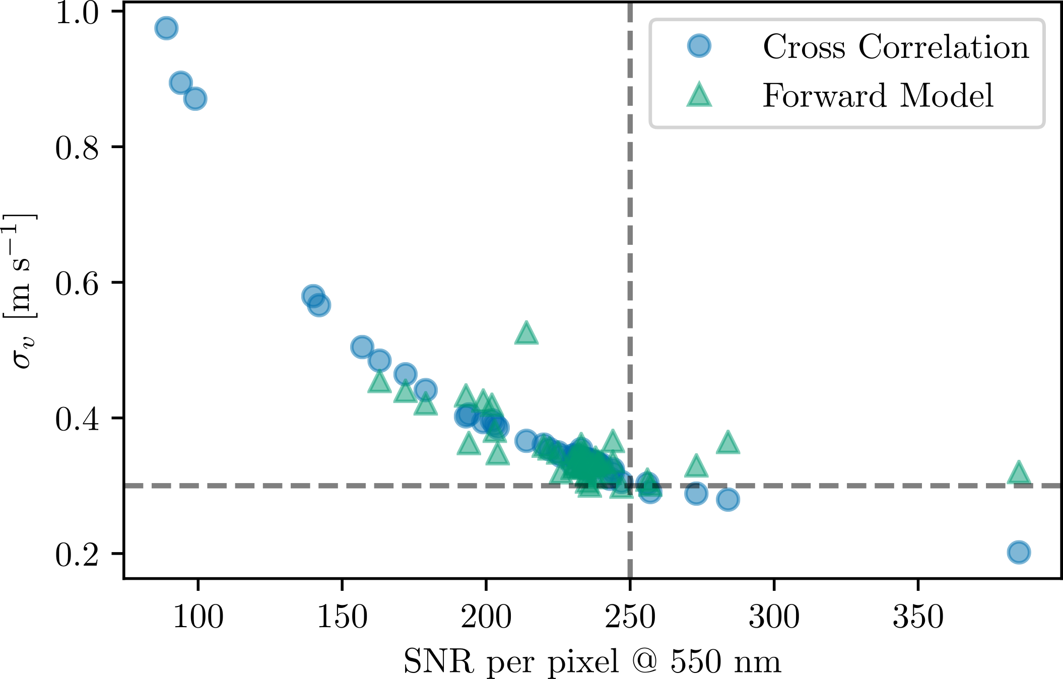
Each EXPRES observation has an approximate per-pixel SNR of 250 at 550 nm, which translates to about 30 cm/s formal RV errors. Most stars have three or four consecutive observations per night, for an equivalent SNR of about 500, and 20+ nights of observations.

Data for HD 101501, which exhibits clear evidence of stellar activity, will be released first to serve as a test case both of the data and project guidelines. Following this test case, data for HD 34411, HD 217014, and HD 10700, including the most up-to-date data collected during the test period with HD 101501.

Data are hosted on Yale Box. Please e-mail Debra Fischer (debra.fischer@yale.edu) and Lily Zhao (lily.zhao@yale.edu) to request access.

1. HD 101501, G8V B, \(log R'_{HK}\) = -4.54
   (45 observations, 22 nights, Feb. 10, 2019 - Nov. 26, 2020)
2. HD 26965, K1V, \(log R'_{HK}\) = -5.01
   (114 observations, 37 nights, Aug. 20, 2019 - Nov. 27, 2020)
3. HD 10700, i.e. tau Ceti, G8V, \(log R'_{HK}\) = -4.98
   (174 observations, 34 nights, Aug. 15, 2019 - Nov. 27, 2020)
4. HD 34411, G0V, \(log R'_{HK}\) = -5.09
   (188 observations, 58 nights, Oct. 08, 2019 - Nov. 27, 2020)

Note: HD 26965 replaced HD 217014 for targets on offer. HD 26965 has more data of higher quality and is more scientifically interesting.

For each star, we offer:

• Raw data upon request
• Meta-data (e.g. airmass, moon distance, etc.), included in the primary FITS extension header
• Telemetry (e.g. temperatures, pressures, etc.) upon request
• Extracted data [9], including
• Wavelengths (+ chromatic barycentric corrected wavelengths [8])
• Flat-relative extracted spectrum
• Continuum model
• Blaze function
• SELENITE telluric model [7]
• Merged 1D Spectra
• Cross-Correlation Functions
• Radial velocities
  • MJD (of the photon-weighted midpoint)
  • Instrument Epoch
  • RVs
  • RV Uncertainties
• Activity indicators
  • S index
  • H-α emission
  • H-α equivalent width
  • Cross correlation function's (CCF) FWHM
  • Measurement of the skew in the CCF's bisector
  • Velocity span of the CCF
  • Asymmetry parameter of a Bi-Gaussian fit to the CCF
  • Asymmetry parameter of a skew normal Gausisan fit to the CCF
• APT photometry [2]

Project Guidelines

To aid the EPRV community in the ever-important fight to disentangle center-of-mass motion (due to planets) from photospheric velocities (due to stellar variability/activity), we will compile a final report of this project. This report will summarize the different methodologies, their relative merits, and their data requirements. In order to analyze the results in a consistent way, we request that for each method, groups submit:

• Activity-adjusted/removed RVs (i.e. cleaned RVs)
• RV signal modeled out as attributed to either activity or noise
• Numerical value of any indicators used
• For GPs: choice of kernel and best-fit hyper parameters

These values will be used to derive the RMS of cleaned, activity-less RVs and the presence (or lack thereof) of activity-driven periodicities for all methods. Participants are encouraged to publish their own papers using the provided EXPRES data and whatever analysis they like.

In working towards a cohesive report and ease of analysis, we provide Submission Guidelines and Method Questions. The Submission Guidelines, which can be found in the following document, specify what each participating group should submit and standardizes file locations, file names, and table structure.

Submission Instructions

We also provide Method Questions to give more detailed information about each method a group tries. These questions focus on 1) a general description of the method, 2) the data requirements for the method, 3) the process of applying the method, and 4) the results of the method. Templates in both LaTeX and Word Document formats are linked below. These templates list all method questions with spaces for answers.

Method Questions [Latex]

Method Questions [Microsoft Word]

Project Timeline

The target submission date for the report is February 2021. Results from each method on all data sets should therefore be submitted by end of December 2020, allowing a month for the report to be written, reviewed, and revised by everyone involved.

Initially, we are providing only the HD 101501 data to serve as a test run, in order to gauge if changes or adjustments are needed of either the data or the project guidelines. The other three data sets, which will include the most up-to-date data, will be made available following this initial run. A detailed timeline is given below.

• Aug. 31, 2020: Information about the project and data links are made public.
• Sept. 14, 2020: Groups must confirm participation by sending a group name, a table of group members, and a rough estimate of number of methods to be tried to Debra Fischer (debra.fischer@yale.edu) and Lily Zhao (lily.zhao@yale.edu).
• Oct. 9, 2020: After some time with the data, a check-in meeting among all participants is held to cover any questions or clarifications concerning the data or the project guidelines.
• Oct. 31, 2020: Groups submit descriptions of all methods and results for HD 101501, revealing any tricks in the data or guidelines and allowing the rest of the project to be more of a treat.
• Nov. 13, 2020: A second check-in meeting is held with all participants to debrief the results of the test run with HD 101501 and identify possible areas for collaboration. Three additional data sets will be released following this meeting.
• Feb. 15, 2021 : Deadline to submit final results/descriptions for all data sets.
• Apr. 6, 2021: A draft of the final report is sent to all participants with a call for feedback. Changes will be made dynamically on the document (on Overleaf) throughout the review period.
• Apr. 20, 2021: A third check-in meeting to discuss conclusions from the project as well as the final report and its scope.
• Oct. 1, 2021: Deadline to give feedback on the paper draft.
• Oct. 22, 2021: A fourth check-in meeting to discuss final changes to the report and future plans for the collaboration.
• Oct. 26, 2021: Report is submitted.

While there are scheduled check-ins for participants to ask questions or raise suggestions, feedback is always welcome and can be sent to Lily Zhao (lily.zhao@yale.edu).

Working with the Extracted Data

The FITS file of each observation contains 3 HDUs. The primary HDU (i.e. index 0) contains the header with documented metadata (e.g. airmass). The first extension HDU (i.e. index 1) contains the optimally extracted data. The second extension (i.e. index 2) contains data from the low-resolution chromatic exposure meter spectrograph and barycentric correction information.

For example, to access the optimally extracted, 2-D spectrum in python, one would use:

>>> hdus = fits.open('file_name.fits')
>>> data = hdus[1].data.copy()
>>> hdus.close()

To read in the same data using IDL:

IDL> data = mrdfits('filename.fits', 1) 
IDL> help, /st, data
** Structure <2806208>, 17 tags, length=799928, data length=799922, refs=1:
   WAVELENGTH      DOUBLE    Array[7920]
   SPECTRUM        DOUBLE    Array[7920]
   UNCERTAINTY     DOUBLE    Array[7920]
   CONTINUUM       DOUBLE    Array[7920]
   OFFSET          DOUBLE    Array[7920]
   OFFSET_UNCERTAINTY
                   DOUBLE    Array[7920]
   N_PIXELS        INT       Array[7920]
   REDUCED_CHI     DOUBLE    Array[7920]
   CONTINUUM_MASK  BYTE      Array[7920]
   PIXEL_MASK      BYTE      Array[7920]
   TELLURICS       DOUBLE    Array[7920]
   ORDER           INT            160
   BARY_WAVELENGTH DOUBLE    Array[7920]
   BLAZE           DOUBLE    Array[7920]
   BARY_EXCALIBUR  DOUBLE    Array[7920]
   EXCALIBUR       DOUBLE    Array[7920]
   EXCALIBUR_MASK  BYTE      Array[7920]

The data variable then contains the following information:

• wavelength gives the wavelengths for each pixel across the entire detector.
• bary_wavelength gives the chromatic-barycentric-corrected wavelengths for each pixel [8]
• spectrum gives the extracted values (Note: the EXPRES pipeline uses a flat-relative optimal extraction method, meaning these values are relative to a flat image constructed for the night. They are therefore unitless and do not correspond directly to any physical properties [9]).
• uncertainty gives errors for each pixel that were propagated through the extraction. As such, when working with continuum normalized spectra, these uncertainties should also be continuum normalized.
• continuum gives a fit to the continuum for each order.
• blaze gives the counts of the median flat exposure that the extractions were done with respect to. Multiplying the spectrum by this blaze will return the original counts for each pixel. These counts, which are presumed Poisson distributed, provide the best measure of SNR for the exposure. Note that because this is simply a median flat exposure, it may contain some detector defects that would otherwise be flat-fielded out in the extracted exposures through the flat-relative extraction. Users are encouraged to fit a smooth function to this blaze before multiplying by the extracted spectrum to recover true counts.
• tellurics gives the SELENITE-constructed telluric model specific to this exposure [7].
• pixel_mask gives a mask that excludes pixels with too low signal to return a proper extracted value. This encompasses largely pixels on the edges of orders. The extracted values for these pixels are set to NaNs.
• excalibur gives the wavelengths generated by Excalibur, a non-parametric, hierarchical method for wavelength calibration <[13]. These wavelengths suffer less from systematic or instrumental errors, but cover a smaller spectral range (~4775-7225 A for epoch 4 and ~4940-7270 A for epoch 5). We have found that the Excalibur wavelengths return RVs with lower scatter.
• bary_excalibur gives the chromatic-barycentric-corrected Excalibur wavelengths for each pixel [8].
• excalibur_mask gives a mask that excludes pixels without Excalibur wavelengths, which have been set to NaNs. These are pixels that do not fall between calibration lines in the order, and so are only on the edges of each order, or outside the range of LFC lines, as described above.

For example, to plot the continuum-normalized spectrum for relative order 66 of EXPRES data in python (which has an index of 65 and corresponds to absolute order 160-65=95), one would use:

>>> plt.errorbar(data['wavelength'][65],
	data['spectrum'][65]/data['continuum'][65],
	yerr=data['uncertainty'][65]/data['continuum'][65])
>>> plt.xlabel('Wavelength [A]')
>>> plt.ylabel('Continuum Normalized Counts')

In IDL:

IDL> wave = data.bary_wavelength              ; chromatic-corrected barycentric wavelengths
IDL> spec = data.spectrum / data.continuum    ; normalized flux 
IDL> unc  = data.uncertainty / data.continuum ; uncertainties for normalized spectrum
IDL> cts  = data.spectrum * data. blaze       ; conts in each pixel
IDL> tell = data.tellurics                    ; SELENITE telluric model
IDL> plot , wave[*, 65], spec[*, 65]          ; to plot order 66 
IDL> oplot, wave[*, 65], tell[*, 65]          ; overplot the telluric model 

This code re-creates the bottom, longer plot in the below figure.

Top left of the above figure plots the spectrum, the returned values from the flat-relative optimal extraction. These values are relative to the median flat for each night and so are unitless with no immediate physical interpretation. Top right shows the spectrum multiplied by the blaze, which recovers the raw, Poisson-distributed counts for each pixel. The bottom plot shows the continuum normalized spectrum from dividing the spectrum values by the continuum fit. Note that similar to the spectrum, one should also divide the uncertainty values by the continuum when working in a continuum normalized regime.

All returned arrays have the format (86, 7920) in python, [7920, 86] in IDL. This corresponds to 86 total orders each with 7920 pixels. The entire EXPRES detector is extracted, giving 7920 pixels in each order. However, in practice, the signal drops off sharply at the edge of each order given the nature of the blaze function. Pixels with too little signal to be extracted are replaced with NaNs in the spectrum and uncertainty arrays (shown as black dots in the above figure). They are masked out by the mask returned by the pixel_mask keyword.

Extracting the full detector also results in many low signal, high uncertainty extracted values on the edges of orders. This can result in noisy even negative extracted values, but ones that are properly associated with huge uncertainties. Therefore, in theory, these points should pose no problem with methods that take the uncertainties into account. In practice, it may be easiest to implement an uncertainty cut on extracted values (i.e. mask out all values with a large fractional uncertainty) as well as masking out the NaN values on either edge of an order.

Meta-Data

Meta-data are contained in the primary HDU's header (i.e. index 0). Keywords for some of the most commonly accessed values are:

• 'AEXPTIME': exposure time of an observation in seconds.
• 'MIDPOINT': geometric midpoint between the shutter opening and closing in UTC time and 'isot' format.
• 'AIRMASS': the average airmass at the center of the exposure, with the beginning and ending airmass given by 'AMBEG' and 'AMEND' respectively.
• 'MOONDIST': distance in degrees from the moon.
• 'SUNDIST': distance in degrees from the sun.

The photon-weighted midpoint is found in the second extension HDU (i.e. index 2) along with other exposure meter data.

• 'HIERARCH wtd_mdpt': photon-weighted midpoint time of exposure.
• 'HIERARCH wtd_single_channel_bc': a single, non-chromatic barycentric velocity value where the velocity is given as a unitless redshift, z=v/c. Note, the bary_wavelength and bary_excalibur keywords in the first extension HDU uses chromatic barycentric corrections.

Line Spread Function (LSF)

The FWHM of an LFC line ranges from 3.9-5 pixels across the detector. More specifically, EXPRES's line spread function can best be represented by either a super-Gaussian or a rectangle (i.e. a top-hat function) convolved with a Gaussian. A super-Gaussian fit tends to behave better because there is less degeneracy at smaller widths. Let a super-Gaussian be defined as:

$$A \, exp \left(-\left(\frac{(x-x_0)^2}{2\sigma_x^2}\right)^P\right)$$

where \(A\) is the amplitude and \(x_0\) is the center of the super-Gaussian. The width \(\sigma_x\) varies smoothly across the detector and is on the order of 1.4 - 2.8 pixels. The exponent, \(P\), ranges between 1 and 2. For more exact PSF parameters across the detector, we are happy to share LFC data for fitting or more specifics about the PSF parameters upon request.

Cross-Correlation Function (CCF)

The CCF for each observation is contained in a FITS File with 3 HDUs. The primary HDU (i.e. index 0) has only a header with relevant meta data (e.g. final calculated velocity and error, other information about the observation). The first extension HDU (i.e. index 1) contains the combined CCF while the second extension (i.e. index 2) contains the order-by-order CCFs.

With the second data release, CCFs have generously been provided by the Penn State team and optimized through work done by Eric Ford, Alex Wise, Marina Lafarga Magro, and Heather Cegla. A standard version of the CCFs that uses ESPRESSO masks, uniform line weights per target, and a CCF mask width tuned to the LSF of EXPRES is distributed. If teams are interested in different variants of the CCF, please contact Eric Ford (eford[at]psu[dot]edu).

The first extension HDU (i.e. index 1) contains the velocity grid on which the CCF is evaluated under the keyword 'V_grid' in units of cm/s and the combined CCF for the observation under the keyword 'ccf', with errors under 'e_ccf'. The overall CCF only combines a subset of orders (relative orders 42-71, which corresponds to absolute orders 89-118), which are orders with high signal and excalibur wavelengths.

The second extension HDU (i.e. index 2) contains the CCFs for each individual order. Each order is evaluated on the same velocity grid as given in the first extension HDU. The CCF values are given under the keyword 'ccfs' with the errors under 'errs'. The velocity and associated error from each order is also given under 'v' and 'e_v' respectively. Note that orders with no signal will have all zeros in place of a ccf.

Radial Velocities

Radial velocities, along with their errors and barycentric midpoint times, are collected in a CSV table for each target along with activity indicators (see below). This same information is also provided in a DACE compatible file. For each observation, two RV measurements are given. CCF RVs are derived using the classic cross-correlation function method of finding RVs. The ESPRESSO mask and line weighting specific to each target star's spectral type is used. For the window function, we use a half cosine.

CBC RVs refer to RVs found using the chunk-by-chunk (CBC) method. Each observation is split up into ~2 A chunks. An RV for each chunk is found by shifting a template spectrum to match the observed spectrum. RVs for each chunk are weighted by how well behaved that chunk is over time and combined to recover an RV for each exposure. The RVs included in the provided data tables were found using 42, 140-pixel-wide chunks in relative orders 43-75 (i.e. index 42-74, absolute orders 118 to 86) ranging from pixel 770 to 6650 across each order. The Excalibur wavelengths were used.

EXPRES data are divided into separate instrument epochs, which demarcate when hardware changes/fixes were implemented. Only data from epochs 4 and 5 are given, which represent post-commissioning EXPRES. Epoch 4 started on Feb. 7, 2019 and continued until Aug. 04, 2019. Epoch 5 started on Aug. 04, 2019 and is the current epoch. Epoch information is included in the radial velocity/activity indicator table. For more information, see Petersburg + 2020, section 3 [9].

Between epoch 4 and epoch 5, the only adjustments were made to the LFC to make it more stable. As a result, the LFC covers a smaller, redder wavelength range in epoch 5 than it did in epoch 4; the LFC ranges from ~4775-7225 A for epoch 4 and ~4940-7270 A for epoch 5. We expect this to have a small effect on the wavelength precision for these orders and changes the range of available Excalibur wavelengths. The changes between epoch 4 and epoch 5 should only affect the wavelength solution, but participants can consider treating the data from different epochs independently.

Activity Indicators

Activity indicators are provided in a table that includes all activity indicators for all observations of a given target along with radial velocity information. They will also be in the first extension HDU's header of each FITS file. Note: missing activity indicator values are replaced by NaNs.

Unless otherwise described, cited errors for each activity indictor is given as the spread in the indicator's values for seven quiet stars for a total of ~400 observations. A histogram of each indicator's values for every observation of those supposed quiet stars was fit to a Gaussian. The width of that Gaussian is reported here as the error.

The S index is given in the FITS headers under the keyword "S-VALUE". This gives the ratio of the Ca II H line core emission to the Ca II K line core emission calibrated to be consistent with the Mt. Wilson Observatory catalog [1]. To build SNR, all exposures taken in a night are combined to find a nightly S-value, which is reported for all observations taken that night. For a number of quiet stars, the spread in the returned S index is 6.611E-3.

The H-alpha core emission is given in the FITS header under the keyword "HALPHA". This represents the ratio of the H-alpha core emission relative to the continuum. The core emission is found as the minimum of the H-alpha line, which has been over-sampled using a cubic spline. The continuum is given as the medium of a nearby, line-less region. The approximate error in the H-alpha core emission value is 1.879E-2 with no real units.

The H-alpha equivalent width is given in the FITS header under the keyword "HWIDTH". This value gives the equivalent width of the H-alpha absorption line. The approximate error for the H-alpha equivalent width is 0.0142 A.

The CCF FWHM (i.e. cross correlation function's full width at half maximum) is given in the FITS header under the keyword "CCFFWHM" (yes, that's two F's in the middle). This value gives the width of the CCF as determined by fitting a Gaussian to the CCF. The error from the covariance matrix of this fit is given in the FITS header under the keyword "CCFFWHME". Empirically, however, the spread in CCF FWHM values for a number of quiet stars is 5.316 m/s.

We determine the bisector of the CCF by finding the midpoint between the left and right wing of the CCF at 100, equally-spaced points ranging from the bottom to the top of the CCF. The "BIS" keyword gives the difference between the mean of the top (60-90 percentile) and the bottom (10-40 percentile) of the CCF bisector (as defined in Queloz+ 2001 [3]). The approximate error of this BIS measurement is 2.515 m/s.

The velocity span of the CCF is defined as the difference in mean of a Gaussian fit to the top of the CCF vs. the bottom of the CCF. Top and bottom points are defined as greater than one sigma away from the center or within one sigma of the center respectively. This value is given in the FITS header under the keyword "CCFVSPAN". The approximate error of this velocity span measurement is 2.297 m/s.

Asymmetry in the CCF is also probed using a bi-Gaussian fit. A bi-Gaussian incorporates an asymmetry parameter in the fit, which can be used as an activity indicator. This value is given in the FITS header under the keyword "BIGAUSS". The approximate error of this bi-Gaussian measurement is 0.168 with no units.

The skew normal similarly gives a measure of asymmetry in the CCF by incorporating a Gaussian model with an inherent asymmetry parameter. This asymmetry value is given in the FITS header under the keyword "SKEWNORMAL". The approximate error of this skew normal measurement is 0.0305 with no units.

APT Photometry

Photometry is from Fairborn Observatory's 0.74-m Automatic Photoelectric Telescopes (APT) in southern Arizona [2]. The APT is equipped with a single-channel photometer that uses an EMI 9124QB bi-alkali photomultiplier tube to measure the difference in brightness between a program star and three nearby comparison stars in the Strömgren b and y passbands.

Photometry is provided in CSV files with three columns. The first column, "Time [MJD]", gives the time of each exposure. The second column, "V [mag]", gives relative magnitudes in the V-band. The last column, "Trend [mag]", represents a model of long-term trends present in the light curve obtained by smoothing the light curve over 100 days [12]. This data are accompanied by a table summarizing the results from individual observing seasons.

Requested Acknowledgements

We are eager to have people from different groups, different countries, and different backgrounds participate. Please let us know (e-mail debra.fischer@yale.edu, lily.zhao@yale.edu) if you plan to publish results using the data made available through this project. We kindly request papers using this data include the below statement in the acknowledgments and cite the following papers.

EXPRES Data Acknowledgment Statement

"These results made use of data provided by the Yale-SFSU-Lowell EXPRES team using the EXtreme PREcision Spectrograph at the Lowell Discovery telescope, Lowell Observatory. Lowell is a private, non-profit institution dedicated to astrophysical research and public appreciation of astronomy and operates the LDT in partnership with Boston University, the University of Maryland, the University of Toledo, Northern Arizona University and Yale University. EXPRES was designed and built at Yale with financial support from MRI-1429365, NSF ATI-1509436 and Yale University. Research with EXPRES is possible thanks to the generous support from NSF 2009528, NSF 1616086, NASA 80NSSC18K0443, NSF AST-2009528, the Heising-Simons Foundation, and an anonymous donor in the Yale alumni community."

Citations

This BibTeX file contains the citations for all articles listed below.

1. Jurgenson+ 2016 [export citation]: the original instrument paper for EXPRES
2. Levine+ 2018 [export citation]: paper describing the status and performance of the Lowell Discovery Telescope
3. Blackman+ 2020 [export citation]: paper assessing instrument performance of EXPRES
4. Petersburg+ 2020 [export citation]: paper describing the extraction pipeline of EXPRES
5. Zhao+ 2021 [export citation]: paper describing the excalibur wavelength algorithm
6. Brewer+ 2020 [export citation]: paper demonstrating EXPRES on-sky precision
7. Zhao+ 2020 [export citation]: research note describing this project, to be cited before the publication of the final report.

Related Papers

1. Zhao, L.L.; Fischer, D.A.; Ford, E.B.; et al. 2022 "The EXPRES Stellar Signals Project II. State of the Field in Disentangling Photospheric Velocities ", AJ, 163, 171
2. Zhao, L.L.; Fischer, D.A.; Ford, E.B.; Henry, G.W.; Rottenbacher, R.M.; Brewer, J.M. 2020 "The EXPRES Stellar-Signals Project I. Data Release", RNAAS, 4, 156
3. Zhao, L.L.; Hogg, D.W.; Bedell, M.; Fischer, D.A. 2020 "Excalibur: A Non-Parametric, Hierarchical Wavelength-Calibration Model for Precision Spectrographs", AJ, 161, 2
4. Cabot, S.H.C.; Rottenbacher, R.M.; Henry, G.W.; Zhao, L.L.; Harmon, R.O.; Fischer, D.A.; Brewer, J.M.; Llama, J.; Petersburg, R.R.; Szymkowiak, A.E. 2020 "EXPRES. II. Searching for Planets Around Active Stars: A Case Study of HD~101501", AJ, 161, 1
5. Brewer, J.M.; Fischer, D.A.; Blackman, R.T.; Cabot, S.H.C.; Davis, A.B.; Laughlin, G.; Leet, C.; Ong, J.M.; Petersburg, R.R.; Szymkowiak, A.E.; Zhao, L.L.; Henry, G.W.; Llama, J. 2020 "EXPRES 1. HD 3651 an Ideal RV Benchmark", AJ, 160, 67
6. Blackman, R.T. (and 27 co-authors) 2020 "Performance Verification of the EXtreme PREcision Spectrograph", AJ, 159, 238
7. Petersburg, R.R.; Ong, J.M.; Zhao, L.L.; Blackman R.T.; Brewer, J.M.; Buchhave, L.A.; Cabot, S.H.C.; Davis, A.B.; Jurgenson, C.A.; Leet, C.; McCracken, T.M.; Sawyer, D.; Sharov, M.; Tronsgaard, R.; Symkowiak, A.E.; Fischer, D.A. 2020 "An Extreme Precision Radial Velocity Pipeline: First Radial Velocities from EXPRES", AJ, 159, 187
8. Blackman, R.T.; Ong, J.M. Joel; Fischer, D.A. 2019 "The Measured Impact of Chromatic Atmospheric Effects on Barycentric Corrections: Results from the EXtreme PREcision Spectrograph", AJ, 158, 40
9. Leet, C.; Fischer, D.A.; Valenti, J.A. 2019 "Towards a Self-Calibrating, Empirical, Light-Weight Model for Tellurics in High-Resolution Spectra", AJ, 157, 187
10. Levine, S.E.; DeGroff, W.T.; Bida, T.A.; Dunham, E.W.; Jacoby, G.H. 2018 "Status and performance of Lowell Observatory's Discovery Channel telescope and its growing suite of instruments", SPIE, 10700, 4PL
11. Blackman, R.T.; Szymkowiak, A.E.; Fischer, D.A.; Jurgenson, C.A. 2017 "Accounting for Chromatic Atmospheric Effects on Barycentric Corrections", ApJ, 837, 18
12. Jurgenson, C.; Fischer, D.; McCracken, T.; Sawyer, D.; Szymkowiak, A.; Davis, A.; Muller, G.; Santoro, F. 2016 "EXPRES: a next generation RV spectrograph in the search for earth-like worlds", SPIE, 9908, 6TJ
13. Queloz, D.; Henry, G.W.; Sivan, J.P.; Baliunas, S.L.; Beuzit, J.L.; Donahue, R.A.; Mayor, M.; Naef, D.; Perrier, C.; Udry, S. 2001 "No Planet for HD 166435", A&A, 379, 279
14. Henry, G.W. 1999 "Techniques for Automated High-Precision Photometry of Sun-like Stars", PASP, 111, 845H
15. Duncan, D.K. (and 17 co-authors) 1991 "Ca II H and K Measurements Made at Mount Wilson Observatory, 1966--1983", ApJS, 76, 383